What is Pearson correlation? Pearson Correlation can be defined as the degree of the linear relationship between two or more sets of variables.
It is used in understanding the energy in the connectivity between variables. Pearson correlation of variables is measured with a statistical term called Correlation Coefficient or Pearson product-moment correlation coefficient.
This term is denoted by a letter r
In statistics, Pearson Correlation between variables x and z can simply be defined as follows:
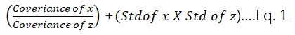
Where Std = Standard Deviation
This also implies that in normally distributed sets of variables, the Pearson correlation coefficient is good for the measurement of covariance of those variables.
Pearson correlation coefficient is not used in the measurement of the degrees of relationship between dependent and independent variables, it does not measure dependent variables neither is it used to measure independent variables.
That is to say that in Pearson correlation, there is nothing like dependent or independent variables. Every variable is equally distributed and as such, they are treated in the same way.
Related Posts:
How To Test Hypothesis In Statistics | A – Z Guides Using Practical Examples
Duncan’s Multiple Range Test On SPSS | A – Z Guides On The Analysis
Measures Of Relationship In Statistics | The Tutorial With Practical Examples
Measurement of Pearson Correlation Coefficient, r
Pearson correlation coefficient is measured statistically in such a way that the value of the r usually run between the value of -n1 and +1. Within this range, the value of r can also be obtained as zero (0).
Let us see what these values really imply here.
| Values of r | Interpretation |
| +1 | Perfect positively correlated |
| -1 | Perfect negatively correlated |
| 0 | Uncorrelated |
| 0.1 – 0.3 | Slightly positively correlated |
| 0.3 – 0.5 | Fairly positively correlated |
| 0.5 – 1.0 | Strongly positively correlated |
| -0.1 to -0.3 | Slightly negatively correlated |
| -0.3 to -0.5 | Fairly negatively correlated |
| -0.5 to -1.0 | Strongly negatively correlated |
Pearson correlation coefficient can be calculated manually or automatically.
The analysis of the Pearson correlation between different variables can effortlessly be run with the help of some statistical tools and software.
A lot of statistical tool have been used to generate accurate result of the Pearson correlation. One of such tool is Microsoft Excel Office.
It quite unfortunate that so many students of statistics and other persons who carry out projects which require Pearson correlation analysis do not know how to use Microsoft Excel to carry out this operation.
It is a very simply and easy task to execute.
In this article, I will be sharing ideas on how you can carry out Pearson correlation analysis on Microsoft Excel. If you have been worried about how you can run Pearson correlation analysis on Excel by yourself, this is the right article that you cannot afford to miss. Kindly stay here and read to the end.
How to Run Pearson Correlation Analysis on Excel
In this section, I will be guiding you on the step by step guide on how to run the Pearson correlation analysis on Excel. Make sure that you follow these procedures if you want to start running your correlation using Excel.
Let us assume that you want to get the correlation between some soil minerals. Here your variables are the given soil minerals that you are working on.
Follow these steps to generate your results.
Step 1: Type your data (the values of the soil minerals) on your Excel worksheet.
Step 2: Go to Data
Step 3: Open data analysis
Step 4: Select Correlation from the Analysis tools and click OK
Step 5: Manually select all your variables on the Excel worksheet
Step 6: Mark the box, “Label in First Row”
Step 7: Click OK to generate your result.
Recommended Posts:
How to Log Transform Data in SPSS
How to Analyze Descriptive Statistics in SPSS
How to Become a Data Analyst | No Certificate is Required
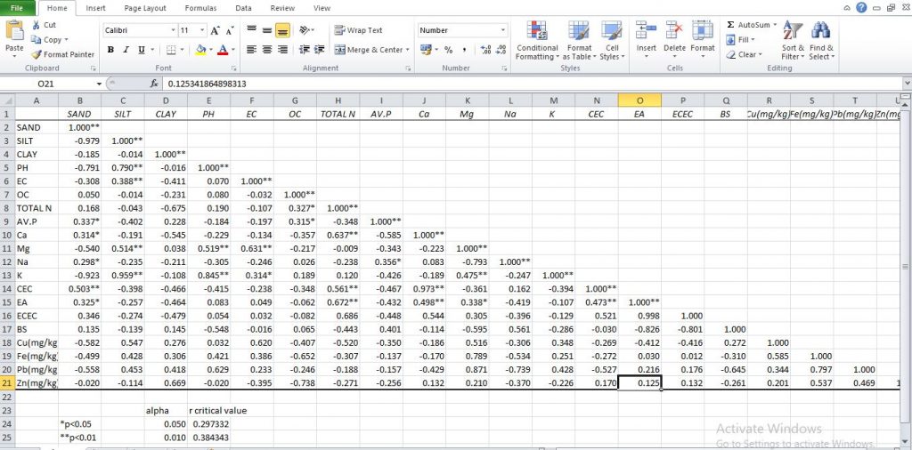
Formatting of Result
After you have generated the result for the correlation analysis from Excel, you still have to make your work look more organised.
To make your result more understandable, you need to show how your variables are correlated, show the significant variables and adjust your values to a definite decimal place.
This is what is regarded as formatting in Excel. There are many ways to format the result that you have generated on your Excel. I am going to take each formatting procedure step by step to help you understand it better.
Adjusting Decimal Places
Assuming that you want all you values to appear in 3 decimal places, this is what you have to do:
- Go to format
- Come down to Format Cell
- Go to Number
- Enter 3 at the space beside Decimal place
- Click Ok, change your values to 3 decimal places
Indicating Significant Values
Your values could be significant at different levels which include; 1%, 5% or 10% probability levels. To show that any of your values are at any of the significant levels, there are different methods to use.
The most frequently used method is the use of asterisks on each of the significant values (e.g: 0.554**, 0.856*). To carry out this operation, you are still going to calculate the significant values.
Are you worried about calculating the significant values? That is very simple to do!
Just keep following this article carefully as I am going to guide you with a simple formula for the calculation of the significant values at any of the probability levels.
What is the first thing for you to do? Go back to your Pearson correlation result on the worksheet and do the following:
The formula is:

…Eq. 2
Where a = Alpha values (0.05 and 0.01)
n = Number of data in the correlation
SR= Square root
Step 1: In two cells, enter *p<0.05 and **p<0.01 respectively.
Step 2: Indicate n value
Step 3: Write down the alpha values
Step 4: Calculate r for a = 0.05 first (you can start with of the alpha values) using eq. 2
Step 5: Use auto sum to get r from the second alpha value.
Step 6: Select your data
Step 7: Go to Conditional formatting
Step 8: come down to the new rule
Step 9: Use “Format any cell that contains”
Step 10: Go to Edit rule description and arrange it as follows:
Cell value >> Between >> r at 0.05 and r at 0.01
Step 11: Click format
Step 12: Change Number to Custom
Step 13: Go to sample and change it to 3 decimal places with the highest number of r, which is the value of r at alpha value 0.01.
Step 14: In general insert 0.000“*” and click Ok. Any value that appeared with one asterisk are significant at *p<0.05 but not at **p<0.01.
To get values which are significant at 0.01;
- Repeat step 6 to step 9 above
- At step 10, change it to r at 0.01 and 1(since 1 is the highest correlation value)
- Repeat step 11 to step 13
- At step 14, enter 0.000 “**”and click Ok. All the values that are significant at 0.01 will be displayed with two asterisks on them.
In case you have a negatively correlated values, you have to multiply you critical value by minus one (-1) and repeat the processes of formatting again.
This is everything that you need to run a Pearson correlation analysis on Excel successfully.
I hope that you have found this article very helpful. Ensure that you use the share button. Do not forget to activate the notification button if really want to be receiving updates on some methods of statistical analysis of this kind.
For any other questionings about Pearson correlation in Excel, kindly use the comment section below.
Please share this article with others if you have found it helpful.