
This article is a special guide on the Measures of Relationship in Statistics. If you would like to be guided on how to handle any measurement of relationship as far as statistics is concerned, this is the article that you must not take for granted.
Are you a student who is handling undergraduate or postgraduate project(s)? I would like to inform you that this article is very important for the analysis and interpretation of your work.
If have been finding it difficult to deal with any calculations that are related to Correlation and Regression, you do not have to worry yourself anymore.
Comprehensive explanations with practical examples have been provided in this article that you are reading. All that you have to do is to ensure that you pay good attention to all information contained therein.
Continue to read further if you are really interested in the guides on measures of relationship in statistics.
Relationship Between Variables
How the distribution of data relates with one another is one of the methods of distinguishing the properties of distribution scores. In this section of the article, I will be discussing how possible variables can relate with one another.
For example, one might be interested to show the relationship between children’s growth per year and the quantity of food taken in a day. Therefore, measures of relationship indicate the degree to which two quantifiable variables are related to each other.
Information on the relationship between the two variables given in the above example could be used to predict how children in a selected area grow if they are fed frequently daily.
The use of such information to describe the magnitude or the degree of the relationship between these variables is very important. Issues such as these are treated under Correlation and Regression.
Correlation Coefficient
Correlation Coefficient can be defined as an index of the degree of linear relationship between two variables. It is represented by the letter r. the measure of Correlation Coefficient ranges from the value, -1.00 to +1.00.
If the variables are not related, the correlation coefficient is usually zero or nearly zero. If they are highly correlated, correlation coefficient of nearly +1.00 and -1.00 is going to be obtained.
Whereas rvalue of 0 to +1 represent positively correlated variables, r value of -1 to 0 shows negatively correlated variables. The strength of positively correlated variable increases from 0 to + and that of negative correlation increases from 0 to -1.
The squared correlation rxy2 (where rxy is the correlation between variables X and Y) indicates the proportion of explained or shared variance. For example, if rxy = 0.70, then X accounts for (0.70)2 = 0.49 or 49% of the variance in Y and vice versa.
Properties of Correlation Coefficient
The following are some of the notable properties of correlation coefficient:
- In interpretation of coefficient of correlation, it is an error to assume that the causation of an effect is caused by the correlation. No such conclusion is automatic.
- Even if the X variable is highly correlated with Y variable, there is likelihood that the same X variable could also be highly correlation with other variables G, H, D and/or more.
- Since interchanging the two variables of concern such as X and Y in the formula does not change the result, it can be said that correlation coefficient is a symmetric measurement.
- Correlation coefficient does not have any unit of measurement and it is not affected by linear transformation such as adding or subtracting constants or multiplying or dividing all values of a variable by a constant.
Forms of Correlation Coefficients
There are different forms of correlation coefficients. However, the type of correlation coefficient to be used is dependent on the nature of the measurement data of the two variables.
With reference to the four measurement scales in statistics which include; Interval, Nominal, Ordinal and Ratio, measurement data can also be dichotomous. That is, Yes versus No, or Boy versus Girl among others.
Interval Data
When data for variables represent interval or ratio level of measurement, it is best to use the Pearson r for the measurement of the correlation. Just like the mean and standard deviation, the Pearson Correlation r takes into consideration the value of every score in both distributions.
Pearson r is given in terms of definition as:
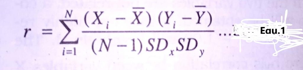
Where, N = Number of cases
SDx = Standard Deviation of X variable
SDy = Standard Deviation of Y variable
The computational formula of the Pearson r is given as:
r =N(∑XY) – (∑X)( ∑Y) …….Equ.2
√{[N∑X2 – (∑X)2][N∑Y2 – (∑Y)2]}
How to Apply the Pearson r Formula
Example: The table below shows the scores of 6 scholars in Physics (X) and Chemistry (Y) promotion examinations. Calculate the Pearson’s Correlation Coefficient between X and Y.
Table 1: table showing the scores of 6 scholars in physics (x) and chemistry (Y) promotion examination.
| Scholars | Physics (X) | Chemistry (Y) |
| 1 | 4 | 3 |
| 2 | 2 | 2 |
| 3 | 5 | 4 |
| 4 | 7 | 3 |
| 5 | 3 | 1 |
| 6 | 2 | 5 |
Solution
Step 1: Try to get the values XY, x2, Y2, and the required summations in a table.
Table 2
| Scholars | X | Y | XY | X2 | Y2 |
| 1 | 4 | 3 | 12 | 16 | 9 |
| 2 | 2 | 2 | 4 | 4 | 4 |
| 3 | 5 | 4 | 20 | 25 | 16 |
| 4 | 7 | 3 | 21 | 49 | 9 |
| 5 | 3 | 5 | 15 | 9 | 25 |
| 6 | 2 | 5 | 10 | 4 | 25 |
| SUMS | ∑X= 23 | ∑Y =22 | ∑XY = 82 | ∑X2 = 107 | ∑Y2 = 88 |
Step 2: Definition of terms
∑X= 23
∑Y =22
∑XY = 82
∑X2 = 107
∑Y2 = 88
Step 3: State your formula
r =N(∑XY) – (∑X)( ∑Y)
√{[N∑X2 – (∑X)2][N∑Y2 – (∑Y)2]}
= (6×82) – (23)(22)
√{[6×10⁷ – 529][6×88 – 484]
= -14
-70.51
r = -0.20
The value the correlation coefficient obtained is -0.20 (negatively correlated). This shows that the result under investigation is linear and it implies that the more the performance of the scholar increases in Chemistry, the more it decreases in Physics.
Ordinal Data
When data for one or both variables are expressed in rank instead of actual scores, then the Spearman’s rho (a form of Pearson correlation) is the best choice to be used in the measurement of the correlation.
Note that the interpretation is the same as previously stated the value of the correlation coefficient ranges from 1.00 to 1.00.
Spearman’s rho rs is represented in formula as shown below:
rs = 1- [6(∑di2)/N3-N]—equ. 3
Where ∑di2 = Sum of squared differences in ranks
N = Number of pair of observations
Example: Suppose two judges ranked the dexterity of five nursing students in handling a thermometer and obtained ranking as shown in the table below. Calculate the rs
Solution
Step 1: Calculate the di and di2 and tabulate your values
Note: The difference in ranking d is obtained by subtracting the ranking of judge I from the ranking of judge II
Table 3:
| Students | Judge I | Judge II | di | di2 |
| 1 | 2 | 5 | -3 | 9 |
| 2 | 3 | 1 | +2 | 4 |
| 3 | 1 | 3 | -2 | 4 |
| 4 | 4 | 2 | +2 | 4 |
| 5 | 5 | 4 | +1 | 1 |
| Total | – | – | – | ∑di2=22 |
Step 2: State your formula and start solving
rs = 1- [6(∑di2)/N3-N]
= 1 – [6×22/53-5]
= 1 – [132/125-5]
= 1 – 132/120
= 1 – 1.1
rs = – 0.1
The relationship between the rankings is low and negative.
Other Forms of Pearson’s Correlation Coefficients
Other forms of Pearson’s correlation coefficients for observed variables include point biserial, Phi coefficient, and rank biserial.
For example, the point-biserial correlation (rpb) is a special case of r that estimates the association between a nominal dichotomous variable and a continuous variable (e.g., gender versus achievement); the phi coefficient (φ) is a special case for two dichotomous variables (e.g. “treatment” versus “control” in experimental studies or the common “Yes” versus “No” response options); the rank biserial correlation (rit) is a special correlation coefficient for the relationship between a nominal dichotomous variable and an ordinal variable.
All forms of Pearson’s correlation coefficient can be estimated by using common statistical packages such as SPSS, SAS and EXCEL.
There are some non-Pearson correlations that assume that the underlying data are continuous and normally distributed instead of discrete. Examples are polyserial, tetrachoric and polychoric correlation coefficients.
The analyses of polyserial, tetrachoric and polychoric correlations are relatively complicated and require specialized software like Linear Structural Relations (LISREL) Version 8, which estimates the appropriate correlations depending on the types of data in the data set.
Linear Regression
The most basic application of regression analysis is the bivariate situation known as linear regression.
Linear regression utilizes the relationship between two variables (one of the variables is termed independent and the other is termed dependent variables) to predict the values or scores of the dependent variable from the independent variable.
For example, to what extent degree does knowledge of the English language (IV) predicts students’ achievement in mathematics (DV)?
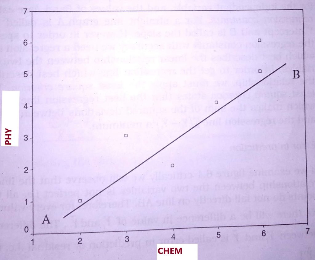
Relationships between the two variables can be examined appropriately by plotting the measurement data on them on a rectangular coordinate system.
The resulting graph is known as a scatter diagram or scatters plot. In plotting the graph the independent variable is denoted by X and the dependent variable is denoted by Y
Figure presented below is a Scatter Diagram of the distribution of six students’ scores in English language X and Mathematics Y. The distribution of the scores is shown in table.
While plotting the scatter diagram, the dependent variable is always placed on the y – axis while the independent variable is placed on the x-axis. Thus, in this example, scores in the mathematics test are placed on the y – axis and scores in the English Language test are placed on the x-axis.
Table 4: Table showing students’ scores in Mathematics and English
| S/N | Mathematics Y | English Language X |
| 1 | 1 | 2 |
| 2 | 2 | 4 |
| 3 | 3 | 3 |
| 4 | 4 | 5 |
| 5 | 5 | 6 |
| 6 | 6 | 6 |
See: How to How to Run Regression Analysis in SPSS
Regression Line and Error in Prediction
Regression Line
In the scatters diagram above, the data appears to be approximated well by the straight line AB.
As a result, we need to determine the equation of the line which best describes the linear relationship between the two variables (i.e. achievement in Mathematics and knowledge of the English Language).
The line which describes the linear relationship between the two variables is called the regression line. To draw the line of best fit for the scatter diagram we need the values of the intercept on the Y axis and the mean of X and Y. Regression line is expressed in the form of a straight line equation
Ȳ=A+BX—-Eqn.4
The variable Ȳ is called predicted Y; X represents the score value for the independent variable, and the values of Band Aare called regression constants.
For a straight-line graph, A is called the Y-intercept and B is called the slope. However, to specify the regression constants with the accuracy we need a regression line that best describes the linear relationship between the two variables.
To get the regression line that best describes the relationship; we must apply the least square criterion. The least-square criterion states that the best regression line is one that makes the sum of the squared deviations between points and the regression line ∑(Yi-Ỹi)2 a minimum.
Error in Prediction
If we examine figure 6.1 critically we will observe that the linear relationship between the two variables is not perfect i.e. all the points do not fall directly on line AB.
Therefore, for every value of Xi, there will be a difference in the value of Yi and Ỹi. The difference between Yi and Ỹi are called error in prediction or residual. i.e. (Yi-Ỹi)2
A measure of the “goodness of the fit” of the regression line to the data is provided by ∑(Yi-Ỹi)2. If this is small, the fit is good; if it is large the fit is bad.
Therefore, in picking the regression line, we go for the situation when ∑(Yi-Ỹi)2 is minimum. The least-squares criterion is satisfied when the sum of the squared deviations between the points and the regression line, ∑(Yi-Ỹi)2 is minimum.
See also: How to Test Hypothesis in Statistics | A-z Guide With Practical Examples
How to Obtain the Regression Line
From equation 4, regression line is expressed in the form of a straight line equation as Ȳ=A+BX. The B in the equation can be calculated using the formula given below:
B = N(∑XY)-( ∑X)( ∑Y)—Equ.5
N ∑X2-( ∑X)2
Example: Calculate the value of B from the table below
Table 5:
| S/N | X | Y | X2 | XY |
| 1 | 1 | 2 | 1 | 2 |
| 2 | 2 | 4 | 4 | 8 |
| 3 | 3 | 3 | 9 | 9 |
| 4 | 4 | 5 | 16 | 20 |
| 5 | 5 | 6 | 25 | 30 |
| 6 | 6 | 6 | 36 | 36 |
| — | ∑X = 21 (∑X)2 = 441 | ∑Y = 26 Ȳ = 4.3 | ∑X2 = 91 | ∑XY = 105 |
| — | Ẍ = 3.5 | – | – | – |
Solution
Using equation 5 above,
B = 6×10⁵ – 21×26/6×91 – 441
= 630 – 546/546 – 441
= 84/105
B = 0.8
To get the Y-intercept A from
Ȳ=A+BẌ…equ.6
Where Ȳ = mean of Yi
Ẍ = mean of Xi
From the table above
Ȳ = 4.3
Ẍ= 3.5
Therefore, A = Ȳ – BẌ
= 4.3 – 0.8 (3.5)
= 4.3 – 2.8
= 1.5
Then the regression equation can be deducted as
Ȳ = 1.5 + 0.8X….Equ.7
Based on the regression equation, it is possible to draw the line of best fit and also predict Y from X. For example, when X = 3, the value of Y can be gotten as follow;
Ȳ = 1.5 + 0.8(3)
= 1.5 + 2.4
= 3.9
From table 5, it is obvious that the predicted value Y (3.9) is greater than (it can be smaller though) the observed value Y (3.0). The difference between the observed Y and the predicted Y is called residual.
Residual = Yi-Ỹi……Equ.8
Table 6: table showing residuals from the regression line
| Ȳ | Ỹi | Yi-Ỹi | (Yi-Ỹi)2 |
| 2 | 3.1 | -1.1 | 1.12 |
| 4 | 4.7 | -0.7 | 0.49 |
| 3 | 3.9 | -0.9 | 0.81 |
| 5 | 5.5 | -0.5 | 0.25 |
| 6 | 6.3 | -0.3 | 0.09 |
| 6 | 6.3 | -0.3 | 0.09 |
Other residuals can be calculated by using equation 8 for each of the other observed values of X. Table 6 shows the observed Yi, the predicted values tilde Y i , as well as the residual for the six observations of Table 5.
The residuals provide an idea of how well the calculated regression line actually fits the data.
The residuals sum of squares (SS) also known as error sum of squares can be expressed as ∑(Yi-Ỹi)2 . From Table 6, the residual sum of squares is 2.94.
From the data in Table 6, it is evident that although we can predict the values of Y using Ȳ=A+BX—-Eqn.4, the predicted value of Y will probably not be equal to the observed value of Y.
It is clear that this predicted value of Y probably will be in error to some extent. It would be useful to have some sort of numerical index to indicate the extent of the error of prediction. The index for indicating the error of prediction is called standard error of estimate (Syx), and it is given by
(S r,X )= √ ∑(Yi-Ỹi)2/ N-2….Equ.9
Standard error of estimate is an index for the variability of Y scores (i. e. ,Yi) . about the regression line
Recommended Links
Duncan’s Multiple Range Test in SPSS software | A-Z Guide on the Analysis
How to Become a Data Analyst Without Any Certificate
How to Analyze Descriptive Statistics on SPSS
How to Log Transform Data In SPSS
Goodness of fit
The line of best fit (on the scatter diagram) is obtained by following these steps. One, determine the intercept A and slope B. This has been shown in the preceding paragraph.
Lay a ruler between the intercept constant on the Y-axis and the point where the (Ẍ and Ȳ), i.e. the mean of Y and X, meet.
Although the regression line is a useful summary of the relationship between two variables, the values of the slope and intercept do little to indicate how well the line actually fits the data. A goodness of fit index is needed.
The observed variation in the dependent variable can be subdivided into two components: these are
- the variation explained by the regression, and
- the residual from the regression.
Total SS=Regression SS + Residual SS
The total sum of squares is a measure of overall variation and is given by
Total sum of squares = ∑(Yi-Ỹ)2…Eqn.10
The regression sum of squares or the sum of squares due to regression is given by
Regression sum of squares = ∑( Ỹi – Ȳ)2 ….Eqn.11
Where
Ỹi is the predicted value for ith case.
The residual sum of square known as error sum of square is given by
Residual sum of squares = ∑(Yi-Ỹi)2…Eqn.12
The regression sum of squares is a measure of how much variability in the dependent variable is attributable to the linear relationship between it and the independent variable.
The proportion of the variation in the dependent variable that is explained by the linear regression is obtained by comparing the total sum of square and the regression sum of squares. It is given by r2
r2 = Regression sum of square/Total sum of square….Equ.13
If there is no linear association in the sample, the value of r2 is 0, since the predicted values are just the mean of the dependent variable and the regression sum of squares is 0.
If Y and X are perfectly linearly related the residual sum of squares is 0 and r2 is 1. The square root of r2 is r, the Pearson correlation coefficient between the two variables.
For the fictitious data on six students (see Table 4), Table 7 below shows the calculation of the regression sum of squares and total sum of squares.
Table 7: Calculation of total and regression sum of squares
| Yi | Ỹi | Yi– Ȳ | Ỹi – Ȳ | (Ỹi – Ȳ)2 | (Yi– Ȳ)2 |
| 2 | 3.1 | -2.3 | -1.2 | 1.44 | 5.29 |
| 4 | 4.7 | 0.3 | 0.4 | 0.16 | 0.09 |
| 3 | 3.9 | -1.3 | -0.4 | 0.16 | 1.69 |
| 5 | 5.5 | 0.7 | 1.2 | 1.44 | 0.49 |
| 6 | 6.3 | 1.7 | 2.0 | 4.00 | 2.89 |
| 6 | 6.3 | 1.7 | 2.0 | 4.00 | 2.89 |
| Ȳ=4.3; ∑(Ỹi – Ȳ)2=11.20; ∑(Yi– Ȳ)2=13.25 |
The regression sum of squares as obtained from Table 6.6 is equal to 11.20, while the total sum of squares is 13.25. The coefficient of correlation for the data is obtained by using Eqn.12:
r2 = Regression sum of square/Total sum of squares
This gives r2 = 11.20/13.25
= 0.85
This shows that there is a high and positive relationship between the two variables. More importantly, 85 % of the variability observed in the mathematics score can be explained by students’ knowledge of English Language.
I believe that you have found this article very helpful. In case of any comment about Measures of Relationship in Statistics, kindly make use of the comment section below this article.
Please do not forget to share this information with others using any of the available social media platforms.